
How to Use ClickHouse Aggregation States to Boost Materialized Views Performance by More Than 10 Times?


In this article, I will discuss how to use Aggregation States in ClickHouse to boost Materialized Views performance by orders of magnitude.
We will be building a small project along the way to show how all different optimizations can work together to achieve high performance guarantees. I will be explaining stuff like: What is ClickHouse? What are Materialized Views and can we use them? What are Aggregation States and how they can make materialized views faster?
Lastly, I will benchmark different approaches using a very large data set (26 billion rows) to show how this optimization can take your data pipeline to the next level.
What is ClickHouse?
ClickHouse is an open-source column-oriented DBMS for online analytical processing that allows users to generate analytical reports using SQL queries in real-time.
Some types of databases are row oriented, in a row-based database, data is laid out on disk as rows, for example, if you have a table with columns (id, name, email), the values for those 3 columns are all stored together in a sequence of bytes representing this row.
On the other hand, columnar databases don’t store all the values from one row together, but store all the values from each column together instead. If each column is stored in a separate file, a query only needs to read and parse those columns that are used in that query, which can save a lot of work. This allows columnar databases, like ClickHouse, to leverage the fact that the data is stored in this fashion to enable features like efficient data compression and vectorized processing.
To learn more about columnar databases, check this article: Designing Data Intensive Applications: Ch3. Storage and Retrieval | Part 2
Problem Description
Let's first set the stage by going over the description of the problem we are trying to solve. Let's assume we are building an internal observability system that stores logs related to services uptime and latency.
So let's assume we have an internal component that periodically pings all services in the system to see if they are alive (a basic health check) and it also records the latency of every ping in order build statistics regarding historical service latency along with some other metadata like if the ping succeeded or not and the instance type used in the service being pinged for example.
Let's assume that this the log format produced by the observability system:
{
  "service_id": 1234, //unique identifier for every service in the sytem
  "timestamp": 1706358554, //timestamp in epoch
  "latency_ms": 3000, //service latency during healthchecks
  "succeeded": true, //represents if this ping was successful or not
  "instance_type": "c5.large" //instance type used in the service
}
System Requirements
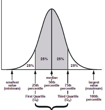
Now let's assume that want this observability system to be able to construct a summary table like the following:
+------------+----------------+----------------+------------+
| service_id | latency_p50_ms | latency_p95_ms | ping_count |
+------------+----------------+----------------+------------+
| 1234       | 3000           | 9000           | 1000000    |
| 4567       | 500            | 1500           | 1254588    |
| 8910       | 1200           | 7200           | 100        |
+------------+----------------+----------------+------------+
which shows for every service, the p50 and p95 for ping latency along with how many times the service was pinged. We would also like to be able to filter this table by metadata, like for example, filtering this table by day, or by the instance type used in the service.
One final requirement is to exclude failing pings from the latency percentilescalculations because they can cause unwanted skew of the numbers, but we want to include them normally in the ping_count
Basic Approach
We can go with a very straightforward approach by creating a ClickHouse table to store the logs as follows (let's assume we will use the MergeTree family):
CREATE TABLE observability.ping_logs
(
    `service_id` UInt8,
    `timestamp` DateTime64(3, 'UTC'),
    `date` Date MATERIALIZED toDate(timestamp),
    `latency_ms` UInt64,
    `succeeded` Bool,
    `instance_type` LowCardinality(String)
)
ENGINE = MergeTree
PARTITION BY toYearWeek(timestamp)
ORDER BY (service_id, succeeded, instance_type, date)
SETTINGS index_granularity = 8192
A couple of things to note here:
I chose the
LowCardinalitysubstructure for theinstance_typecolumn because reasonably a system would have a few different instance types (let's assume we are only using the C family instances for the sake for this article). TheLowCardinalitysubstructure enables dictionary encoding for the underlying data type (similar to Enum) which works very well for columns with less than 10,000 possible values. For more details refer to the docs.Similarly, since a normal system wouldn't have a ton of services, I chose
UInt8which will support to 256 possible values which seems reasonable for this usecase. But why didn't we use theLowCardinalitysubstructure here as well to enable dictionary encoding? Because it's prohibited by default by ClickHouse due to its expected negative impact on performance.I chose to partition the table by week of the log timestamp because:
This will optimize queries by pruning partitions that don't belong in the search space (for usecases like filtering by timestamp).
This will produce a manageable number of partitions which is important for ClickHouse (you can't use an expression that will produce too many partitions, because it will produce too many parts during inserts).
I add an extra materialized column called
datewhich is just the conversion of the timestamp to day, this is because, we only want to query logs by day, we don't need to query by hour for example and adding this column in theORDER BYclause beforetimestampwill help speed up queries.Notice the order of columns in the
ORDER BYclause, they are "mostly" ordered by least cardinality to highest (from left to right) which is important to be able to serve as many query patterns as possible efficiently.- Note that although
service_iddoes have a higher cardinality than other columns to its right, it was still placed at the beginning because under our system's definition it will always be included in all query patterns, so it doesn't really matter where to place it.
- Note that although
Now let's insert some rows into our table:
┌─service_id─┬───────────────timestamp─┬─latency_ms─┬─succeeded─┬─instance_type─┐
│          1 │ 2024-01-03 00:00:00.000 │      17000 │ false     │ c5.large      │
│          1 │ 2024-01-01 00:00:00.000 │       3000 │ true      │ c5.large      │
│          1 │ 2024-01-01 00:00:00.000 │       3500 │ true      │ c5.large      │
│          1 │ 2024-01-02 00:00:00.000 │       5000 │ true      │ c5.large      │
│          2 │ 2024-01-01 00:00:00.000 │        300 │ true      │ c5.xlarge     │
│          2 │ 2024-01-01 00:00:00.000 │        303 │ true      │ c5.xlarge     │
│          2 │ 2024-01-01 00:00:00.000 │        307 │ true      │ c5.xlarge     │
│          2 │ 2024-01-01 00:00:00.000 │        502 │ true      │ c5.xlarge     │
│          3 │ 2024-01-02 00:00:00.000 │      60000 │ false     │ c5.4xlarge    │
│          3 │ 2024-01-02 00:00:00.000 │      60000 │ false     │ c5.4xlarge    │
│          3 │ 2024-01-02 00:00:00.000 │      60000 │ false     │ c5.4xlarge    │
└────────────┴─────────────────────────┴────────────┴───────────┴───────────────┘
To build the table we mentioned previously, we can use a query like this:
SELECT
    service_id,
    quantilesTDigestIf(0.5)(latency_ms, succeeded = true) AS latency_p50_ms,
    quantilesTDigestIf(0.95)(latency_ms, succeeded = true) AS latency_p95_ms,
    count(*) AS ping_count
FROM observability.ping_logs
GROUP BY service_id
ORDER BY ping_count DESC
Which will produce the following result for the data set we have:
┌─service_id─┬─latency_p50_ms─┬─latency_p95_ms─┬─ping_count─┐
│          1 │ [3500]         │ [5000]         │          4 │
│          2 │ [303]          │ [502]          │          4 │
│          3 │ [nan]          │ [nan]          │          3 │
└────────────┴────────────────┴────────────────┴────────────┘
Notice the following:
I chose to use the
quantilesTDigestbecause it's very space efficient for large data sets (this is crucial in a production system), it uses \(O(logN)\) space for an \(N\) rows data set.I used the
Ifcombinator to add an extra condition to the calculation of percentiles to only consider successful pings as the requirement states. The beauty of this is that only affects the percentiles calculations but nothing else in the result, for example,ping_countwould still show count of both successful and failing pings (instead of going through the hassle of doing this using sub-queries), you can see this in service number 1 and 3 because service number 1 had a failing ping with large latency (17,000 ms) which would have definitely skewed the p95 but it didn't because it was excluded. It's even clearer for service 3 whose pings are all failing that's why we gotnanfor percentile values (which we can convert to anything else using combinators as well) andpings_countis reflected normally. For more info regarding how to use combinators, refer to this.
Now this is all good and working, but when the system has billions of logs, things will start to run very slowly. So let's see how can we make this faster?
Enters Materialized Views
Now it's a good time to introduce materialized views into the system and explain what they are. A materialized view is basically a way to incrementally aggregate data on-write to make the data set smaller so when we fire read queries they would run faster.
Let's go over an example to see this in action. The simple way to utilize a materialized view here is to try think of the data set as the combinations of possible values of all columns.For example, what if we group all successful logs from the same service, at the same day and same instance type, with similar latency into a single row?
Let's assume we defined the following materialized view using the TO format, by creating the following data table in which we will store the aggregates:
CREATE TABLE observability.ping_logs_counts_data
(
    `service_id` UInt8,
    `date` Date,
    `latency_ms` UInt64,
    `succeeded` Bool,
    `instance_type` LowCardinality(String),
    `count` UInt64
)
ENGINE = SummingMergeTree
PARTITION BY toYearWeek(date)
ORDER BY (service_id, succeeded, instance_type, date, latency_ms)
SETTINGS index_granularity = 8192
Note that we are now using a SummingMergeTree which is designed for incremental aggregations. And we also added an extra column count to represent how many rows belong to every combination of data.
Now let's create the materialized view that will populate this table as follows:
CREATE MATERIALIZED VIEW observability.ping_logs_counts TO ping_logs_counts_data
AS SELECT
  service_id,
  toDate(timestamp) as date,
  round(latency_ms, -1) as latency_ms,
  succeeded,
  instance_type,
  count(*) as count
FROM observability.ping_logs
GROUP BY
  service_id,
  date,
  latency_ms,
  succeeded,
  instance_type
This will run with every new insert into the ping_logs table and populates the materialized view data table using the defined query here. Note the following:
We convert the timestamp to
Datesince we only ever query the system by date. This is very useful to drop cardinality of the date column, for example, there are 365 days in a year vs billions of millisecond in a year.I am also rounding the
latency_msto the nearest tenth of millisecond, so for example, values like 301 ... 304 will be rounded down to 300, and values from 305 ... 309 will be rounded up to 310 and so on. This is also meant to reduce candinality as much as we can.The rest of the columns are already low cardinality and there is nothing we can do about them.
We had to add
latency_msto the sort key of the materialized view data tableping_logs_counts_databecause summing merge trees replaces all rows with the same sort key with the summarized values and we don't want to sum the values oflatency_msbecause that doesn't make sense, we only want to have a count per combination.
Now let's re-insert our data and see how the materialized view looks like:
┌─service_id─┬───────date─┬─latency_ms─┬─succeeded─┬─instance_type─┬─count─┐
│          1 │ 2024-01-03 │      17000 │ false     │ c5.large      │     1 │
│          1 │ 2024-01-01 │       3000 │ true      │ c5.large      │     1 │
│          1 │ 2024-01-01 │       3500 │ true      │ c5.large      │     1 │
│          1 │ 2024-01-02 │       5000 │ true      │ c5.large      │     1 │
│          2 │ 2024-01-01 │        300 │ true      │ c5.xlarge     │     2 │
│          2 │ 2024-01-01 │        310 │ true      │ c5.xlarge     │     1 │
│          2 │ 2024-01-01 │        500 │ true      │ c5.xlarge     │     1 │
│          3 │ 2024-01-02 │      60000 │ false     │ c5.4xlarge    │     3 │
└────────────┴────────────┴────────────┴───────────┴───────────────┴───────┘
As we can, the materialized view has 8 rows vs 11 rows in the original table. We can see the count of every combination in the count column, like for example, for service 2, the two logs with latency 300 and 303 got grouped together in a single row with the value 300. Similarly for service 3 logs, all logs had the same latency, so they got replaced with a single row in the materialized view with count 3.
The savings here might seem insignificant, but for a production application, this can be 100 times smaller than the original table and thus 100 times faster to query than the original table (we go over this in more details in the benchmarks section).
We can construct the same output table we want using the following query:
SELECT
    service_id,
    quantilesTDigestWeightedIf(0.5)(latency_ms, count, succeeded = true) AS latency_p50_ms,
    quantilesTDigestWeightedIf(0.95)(latency_ms, count, succeeded = true) AS latency_p95_ms,
    sum(count) AS ping_count
FROM observability.ping_logs_counts
GROUP BY service_id
ORDER BY ping_count DESC
and we will get the following result:
┌─service_id─┬─latency_p50_ms─┬─latency_p95_ms─┬─ping_count─┐
│          1 │ [3500]         │ [5000]         │          4 │
│          2 │ [310]          │ [500]          │          4 │
│          3 │ [nan]          │ [nan]          │          3 │
└────────────┴────────────────┴────────────────┴────────────┘
Note the following:
We are now using
quantilesTDigestWeightedIfinstead ofquantilesTDigestIfbecause we are now querying already aggregated in the materialized view instead of raw values from the original table. For example, a row in the materialized view with latency value 300 and count value 2, is basically 2 rows in the main table each having the value 300, so this function enables TDigest to add a weight to each value consistent with how many times it was seen.Similarly, we are using
sum(count)instead ofcount(*)to calculate thepings_countbecause we want to sum the already aggregated rows in the materialized view to get the actual count of the data it stores, not the count of its own rows (which is irrelevant in this context).We notice that the final result is a bit different than what we previously had, this mainly because:
In the materialized view we rounded the value of the
latency_msso it's a little less accurate now (by design).The weighted version of
TDigestis also less accurate (because it's an extra approximation) specially for small data sets.
Now we have an approach that can perform way better than the original approach.
Enters Aggregation States
Now let's assume that even after the previous optimization, performance is still bad. What can we do?
Let's make some observations related to our last approach:
The efficiency of the approach is directly proportional to the size of the materialized view, the smaller can make it, the faster it will be.
The size of the materialized view is directly proportional to the cardinality of the columns included in the
GROUP BYclause (which represents how many combinations are stored in the materialized view).Now let's do some cardinality analysis on the columns we have:
service_id,succeeded,instance_type: should have a few values and there is nothing we can do about this, for example, there is nothing to round or truncate or remove.date: it also has a few values but we can for example round it to week or month to make the cardinality even smaller, however this will badly affect the system, so let's skip that.latency_ms: this is the highest cadinality column we have even after rounding. And we have rounded it enough already.
The key observation here is that the only use for the column
latency_mstocalculate percentiles. **We are not actually using the raw values of the column anywhere (**for example, we don't have a filter on it or display the raw value anywhere). So if we can somehow remove thelatency_msfrom theGROUP BYclause while still being able to calculate percentiles, that will reduce our materialized view by orders of magnitude which will improve performance a lot.
ClickHouse supports something called AggregateFunction which allows working with aggregation states instead of scaler values. To understand this better, let's take a very hypothetical example of calculating the number of unique values in a data set.
Let's assume that we are getting the values of the data set online (one or a few rows at a time), so for example:
Say we received the following values
[1, 2, 3, 2]We construct an array containing the unique values only, so
[1, 2, 3]and save this array internally. This is called an aggregation state, because we have the actual current state of the aggregation. This is opposed to the actual value of the aggregation which is currently 3.Now let's say we received a new batch of values,
[2, 5, 3, 5, 5], we calculate the unique state from this batch, so it's[2, 5, 3]and now we merge this state with the previous state, so we get[1, 2, 3, 5]and now the aggregation value became 4 and so on.
The key observation here is that in order to be able merge states, the state has to contain all the metadata needed to represent that state of aggregation at that point of time. Like for example, if the state is just the value of the aggregation, the first state will be 3 and we can't merge this to the next state, because we don't know what are the 3 values in order to deduplicate.
Disclaimer: this is not how unique aggregation states work, they usually use algorithms like HLL (hyper-log-log) which can approximate the number of unique values in an array without storing the actual values. We won't get into that in this article, this was just an example to explain how aggregation states roughly work.
Pretty much the same happens with TDigest except it's a lot more complicated. It basically operates like a k-means clustering where the data set is split into smaller groups and centriods are calculated for each group and then those centriods are merged together to produce an approximation for quantiles.
Luckily for us, this doesn't require the state to store all the data that was inserted (otherwise it would be infeasible), so we don't have to store the raw values anymore and it can be replaced by storing the aggregation state, so we can remove the latency_ms column from the GROUP BY clause from the materialized view which will bring down the size by orders of magnitude. It's also usually smaller in terms of disk storage.
Let's create new materialized views as follows:
CREATE TABLE observability.ping_logs_counts_data_new
(
    `service_id` UInt8,
    `date` Date,
    `latency_ms` AggregateFunction(quantilesTDigestIf(0.5, 0.95), UInt64, UInt8),
    `succeeded` Bool,
    `instance_type` LowCardinality(String),
    `count` UInt64
)
ENGINE = SummingMergeTree
PARTITION BY toYearWeek(date)
ORDER BY (service_id, succeeded, instance_type, date)
SETTINGS index_granularity = 8192
In the data table we just changed the type of latency_ms from UInt64 to AggregateFunction in order to be ready to store the aggregation state instead of the raw value. And we removed the latency_msfrom the sorting key because nowlatency_msis an aggregation and we want theSummingMergetreeto summarize this column as well for the same sorting key (based on the remaining columns in the sorting key).
And the materialized view definition will be as follows:
CREATE MATERIALIZED VIEW observability.ping_logs_counts_new TO observability.ping_logs_counts_data_new
AS SELECT
  service_id,
  toDate(timestamp) as date,
  quantilesTDigestIfState(0.5, 0.95)(latency_ms, succeeded = true) AS latency_ms,
  succeeded,
  instance_type,
  count() as count
FROM observability.ping_logs
GROUP BY
  service_id,
  date,
  succeeded,
  instance_type
Note that we replaced the latency_ms calculation with an aggregation state that precomputes p50 and p95 based on the condition on-write. I also ditched the rounding logic because it's not needed anymore and we can have better accuracy without affecting the materialized view size. Also since the state will contain data from every single value that we insert, we no longer to consider theweightas we did before, so we can use quantilesTDigestIf instead of quantilesTDigestWeightedIfwhich has an even higher accuracy, so all the better.
There is one important caveat to this approach to note here, is that because now we are calculating the aggregation on write time, we need to provide the condition used for thequantilesTDigestIfin the materialized view definition. So this will work pretty well for static conditions like in this example, but if your conditions can differ at run time, this will not work, however, you might still be able to get around this using sub-queries and common table expressions, albeit a lot more complex.
Now let's re-insert our data and see how the new materialized view looks like:
┌─service_id─┬───────date─┬─latency_ms───────────┬─succeeded─┬─instance_type─┬─count─┐
│          1 │ 2024-01-03 │                      │ false     │ c5.large      │     1 │
│          1 │ 2024-01-01 │ �;E�?�ZE�?           │ true      │ c5.large      │     2 │
│          1 │ 2024-01-02 │ @�E�?                │ true      │ c5.large      │     1 │
│          2 │ 2024-01-01 │ �C�?��C�?��C�?�C�?   │ true      │ c5.xlarge     │     4 │
│          3 │ 2024-01-02 │                      │ false     │ c5.4xlarge    │     3 │
└────────────┴────────────┴──────────────────────┴───────────┴───────────────┴───────┘
We can notice the following:
The new materialized view has 5 rows, compared to 8 rowsfor the old materialized view. This is because the
latency_msis no longer in theGROUP BYso for example, we can see for service 2, a single row containing data for 4 logs is representing the whole aggregate state.The column
latency_mscontains a serialization of the aggregate state instead of a scaler value.Since our aggregation state is conditional on the success of the ping log, rows with only failing pings don't have a state at all.
We will now have to adjust the query we use to construct our output table to be able to work with aggregation states, it will look like this:
SELECT
    service_id,
    quantilesTDigestIfMerge(0.5, 0.95)(latency_ms)[1] AS latency_p50_ms,
    quantilesTDigestIfMerge(0.5, 0.95)(latency_ms)[2] AS latency_p95_ms,
    sum(count) AS ping_count
FROM observability.ping_logs_counts_new
GROUP BY service_id
ORDER BY ping_count DESC
which will produce the following result:
┌─service_id─┬─latency_p50_ms─┬─latency_p95_ms─┬─ping_count─┐
│          1 │           3500 │           5000 │          4 │
│          2 │            303 │            502 │          4 │
│          3 │            nan │            nan │          3 │
└────────────┴────────────────┴────────────────┴────────────┘
We can notice the following:
We had to use the
Mergecombinator to merge aggregation states during query time. Note that aggregation states already get merged in the background during regular merges, but aMergeon read time is still required because background merges only merge states with the same sorting column, while during reads, you might want to handle this differently.We are getting the same result as the basic approach because we ditched rounding and we are not using the weighted TDigest approximation anymore.
So we are no basically getting the same results as approach 1 but much much faster and using a lot less space than approach 2.
Real Life Benchmarks and Accuracy
The example discussed here is more of a toy problem. This approach was tried on a large production system to validate accuracy and benchmark performance.
The table under test contains 26 billion rows of data, here are some results:
Accuracy
The following shows an accuracy test run on a table of size
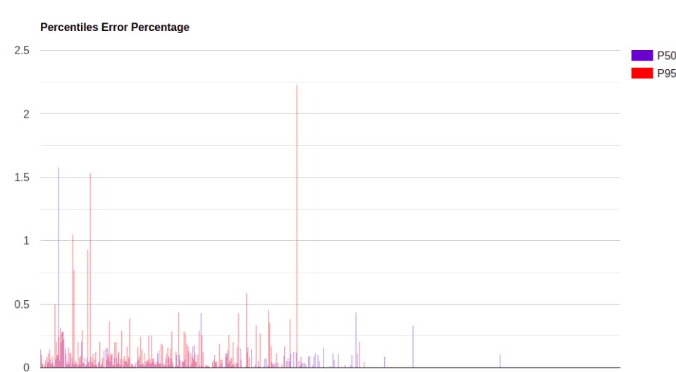
This a test calculating percentiles (p50 and p95) using approach 2 and approach 3 and comparing the accuracy. We can see that for almost all data points, the error for P50 is less than 0.25% with occasional spikes max at 1.5%. For P95 most data points have error percentage less than 0.5% with some occasional spikes up to 2.5%.
This error margin seems acceptable and it's expected that higher percentiles are less accurate for algorithms like TDigest because there are usually less centriods representing them (for a normally distributed data set), because there is less data in those extreme quantiles.
Performance
While running the same query to construct the previously mentioned summary table on both materialized views from approach 2 and 3, we get the following:
Approach 2 (without aggregate function): 11.527 sec and the query processed 430 million rows.
Approach 3 (with aggregate function): 0.797 sec and the query only processed 1 million rows.
For the sake of showing that approach 2 is already a very large optimization, I run the same query on the original table and we get 693.587 sec and it processed the entire table, all 26 billion rows.
Conclusion
When dealing with large data sets for the purpose of analytics, you really need to carefully think about your specific use case because based on your use case, you might be able to unlock some very good optimizations. It's also recommended to start experimenting with trade offs, like for example, rounding some data and losing accuracy for the sake of better performance.
There is no one solution fits all, but there are some guidelines you can follow which I hope that this article helps introduce some new ideas into everyone's thought process.
Credits
Cover picture credits goes to https://clickhouse.com