In the previous article, we discussed the first part of chapter 2 of Designing Data Intensive Applications by Martin Kleppmann. We talked about data models and how they affect the design of any application and compared the relational and the document data models.

In this article, we will continue to explore the rest of this chapter where we will discuss different types of query languages such as, declarative and imperative query languages along with some hybrid languages like MapReduce that combine both approaches to offer more flexibility. We will also introduce some graph-like data models and see how they can represent very complicated and interconnected relationships between data entities via a detailed example.

Query Languages for Data

A data model is just an abstraction of data is represented and stored but this not the whole story, often we will need to query the data we stored and for that we need a query a language which acts as a means of communication with the data store to interact with data.

When the relational data model was introduced, it was introduced with a query language that we all know as SQL (Structured Query Language). SQL is a declarative query language and to know what that means we will have to also consider imperative query languages.

Most commonly used programming languages are imperative which means that you write the logic of the operation (even if you're using a third party helper, after all, the helper was also written imperatively by someone else). For example, if have a collection (a table) called animals and we want to fetch animals that are sharks for this table. In an imperative query language, it will look something like this:

def getSharks()
  sharks = []

  animals.each |animal| do
    if animal.family == 'Sharks'
      sharks << animal
    end
  end

  return sharks
end

What this simple ruby snippet does is that it imperatively describes the exact needed steps to fetch sharks, for examples, it's says, alright, we need to iterate over all records in the animals table, and for each record, we will need to check if it's a shark and if it's a shark, then we add to our result set.

In a declarative language however, like relational algebra (upon which SQL is built), we would write something like this instead:

\(sharks = \sigma_{family='Sharks'}(animals)\)

where \(\sigma\) (the Greek letter sigma) is the selection operator, returning only those animals that match the condition \(family = 'Sharks'\).

When SQL was defined, it followed the structure of the relational algebra fairly closely:

SELECT * FROM animals WHERE family = 'Sharks';

In a declarative query language, like SQL or relational algebra, you just specify the pattern of the data you want—what conditions the results must meet, and how you want the data to be transformed (e.g., sorted, grouped, and aggregated)—but not how to achieve that goal. It is up to the database system’s query optimizer to decide which indexes and which join methods to use, and in which order to execute various parts of the query.

As we can probably see from the above example, declarative languages are not just way more concise, but they are more generic and abstract as it allows the query engine to act independently of queries. For example, if you write an imperative query like the one we wrote to fetch sharks, you might write your query in a way that assumes a certain ordering of data for example in which case the database can never be sure about the assumptions your imperative code is making in order not to break them, unlike the declarative query language.

Furthermore, declarative languages lend themselves to parallel processing a lot more because it's up to the engine to understand what you're trying to do and parallelize it unlike imperative code that would have to parallelized by the programmer who wrote it because it's not generic enough.

MapReduce Querying

MapReduce is a programming model for processing large amounts of data in bulk across many machines, popularized by Google. A limited form of MapReduce is supported by some NoSQL datastores, including MongoDB and CouchDB, as a mechanism for performing read-only queries across many documents.

The idea of map-reduce queries is that it adds some flexibility to the application developer to control the logic a database performs in an imperative way. So you can think of it as a language that's in-between declarative languages and imperative languages in the sense that it still execute declarative queries but it allows application developers to inject some imperative logic.

Let's consider the same example we discussed before, let's furthermore assume that the animals table has a timestamp field that records where a sighting of this specific animal occurred and we don't just want to fetch sharks form the table, rather we want to fetch how many sharks we sighted per month.

A normal SQL query to do this will look like so:

SELECT date_trunc('month', observation_timestamp) AS observation_month,
              sum(num_animals) AS total_animals
FROM observations
WHERE family = 'Sharks'
GROUP BY observation_month;

This query first filters the observations to only show species in the Sharks family, then groups the observations by the calendar month in which they occurred and finally adds up the number of animals seen in all observations in that month.

The same can be expressed with MongoDB’s MapReduce feature as follows:

db.observations.mapReduce(
    function map() {
      var year = this.observationTimestamp.getFullYear();
      var month = this.observationTimestamp.getMonth() + 1;
      emit(year + "-" + month, this.numAnimals);
    },
    function reduce(key, values) {
      return Array.sum(values);
    },
    {
      query: { family: "Sharks" },
      out: "monthlySharkReport"
    }
);

Let's analyze this query to understand the concept of MapReduce better:

1. This query: { family: "Sharks" } part of the query is a declarative part, telling the database that we want to filter documents that are sharks.
2. The function map() is executed once with every document that should end up in the result set (i.e. those documents filtered by the query in step 1, the shark documents) and this function basically converts the observationTimestamp to a string of year-month, for example 2022-01 and it emits that key along with the value of the number of animals in that observation, so it mapped this document to only what we need in the correct format.
3. The function reduce receives the key-value pairs emitted by map() and groups them by key (i.e. the string representing the observation date) and then it aggregates (reduces) the values (in this case it sums the number of observations).
4. Then this result is generated as a monthlySharkReport.

The map and reduce functions are somewhat restricted in what they are allowed to do. They must be pure functions, which means they only use the data that is passed to them as input, they cannot perform additional database queries, and they must not have any side effects. These restrictions allow the database to run the functions anywhere, in any order, and rerun them on failure. However, they are nevertheless powerful: they can parse strings, call library functions, perform calculations, and more.

The idea of MapReduce is very useful and many datastores started to standardize it via builtin pipelines, like for example aggregations pipelines in MongoDB or in Elasticsearch and both still support the concept of injecting custom map/reduce functions to be executed by the engine. For example, the same query above can be written in MongoDB using aggregations pipelines as follows:

db.observations.aggregate([
     { $match: { family: "Sharks" } },
     { $group: {
       _id: {
         year: { $year: "$observationTimestamp" },
         month: { $month: "$observationTimestamp" }
       },
      totalAnimals: { $sum: "$numAnimals" }
     }}
]);

Which is a very similar look to what you would write in other datastores like Elasticsearch for example.

Graph-Like Data Models

We saw in the previous part of this article that the relationships between your data entities might make one data model more appropriate than another, for example, if you're application is mainly consisting of one-to-many relationships (i.e. it can be modeled as a tree) then you would usually want to operate on a subset of this tree at once (for example fetch a Linkedin user and all positions he has), then the data model is more appropriate.

But if your data has more complex many-to-many connections, then the relational model can handle the simple cases of this. But as more complex those interconnected relationships gets, it starts to make a lot more sense to model your data as a graph.

A graph is a data structure consisting of vertices (nodes or entities) and edges (connections). Typical example of graphs are:

• Social graphs: Vertices are people, and edges indicate which people know each other.
• The web graph: Vertices are web pages, and edges indicate HTML links to other pages.
• Road or rail networks: Vertices are junctions, and edges represent the roads or railway lines between them.

Mapping data in a graph model doesn't just make it easier to represent and reason about but it makes it possible for this data to lend itself easily to well-known, specialized algorithms that perform certain functions. Like for example, a shortest path algorithm to calculate the shortest distance between 2 railway stations in a rails network graph or a page rank algorithm to calculate a webpage's popularity in a web graph.

Moreover, data graphs don't have to be homogeneous, for instance, in the previous examples, all data are the same, all vertices are junctions and all edges are roads. But the graph model is powerful enough to represent non-homogeneous data, like for example, some vertices might be junctions and some might be railway stations, some edges might be roads and some edges might represent time for example.

The most popular example for a non-homogeneous graph data model is that run by Facebook, which maintains a single graph with many different types of vertices and edges: vertices represent people, locations, events, checkins, and comments made by users; edges indicate which people are friends with each other, which checkin happened in which location, who commented on which post, who attended which event and so on.

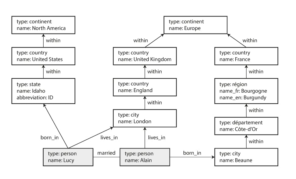
Now let's consider an example to understand the power presented by the graph model. Consider the following data graph:

Data in the graph model can either be represented in one of two models:

Property graphs:

In the property graph model, each vertex consists of:

• A unique identifier
• A set of outgoing edges
• A set of incoming edges
• A collection of properties (key-value pairs)

Each edge consists of:

• A unique identifier
• The vertex at which the edge starts (the tail vertex)
• The vertex at which the edge ends (the head vertex)
• A label to describe the kind of relationship between the two vertices
• A collection of properties (key-value pairs)

Triple store model:

The triple-store model is mostly equivalent to the property graph model, using different words to describe the same ideas. In a triple-store, all information is stored in the form of very simple three-part statements: \((subject, predicate, object)\). For example, in the triple \((Jim, likes, bananas)\), Jim is the subject, likes is the predicate (verb) and bananas is the object.

The subject of a triple is equivalent to a vertex in a graph. The object is one of two things:

1. A value in a primitive datatype, such as a string or a number. In that case, the predicate and object of the triple are equivalent to the key and value of a property on the subject vertex. For example, \((lucy, age, 33)\) is like a vertex lucy with properties {"age":33} like in the property graph model.
2. Another vertex in the graph. In that case, the predicate is an edge in the graph, the subject is the tail vertex, and the object is the head vertex. For example, in \((lucy, marriedTo, alain)\) the subject and object lucy and alain are both vertices, and the predicate marriedTo is the label of the edge that connects them.

For the sake of this example, we will consider the property graph model because it's the closest to a relational model. Now let's say we want to be able to represent the same data model in the previous figure but in a relational database, can we do that?

The answer is yes, but it will be complicated, let's see how:

First we will have to create the needed tables to represent the graph model. For this we chose the property model because it lends itself to the relational model more naturally than the triple store model. So the tables will look like this:

CREATE TABLE vertices (
   vertex_id integer PRIMARY KEY,
   properties json
);

CREATE TABLE edges (
   edge_id integer PRIMARY KEY,
   tail_vertex integer REFERENCES vertices (vertex_id),
   head_vertex integer REFERENCES vertices (vertex_id),
   label
   text,
   properties json
);

CREATE INDEX edges_tails ON edges (tail_vertex);
CREATE INDEX edges_heads ON edges (head_vertex);

As you can we see created tables the represent the property model as explained above and we created indexes on tail_vertex and head_vertex in the edges table to be able to efficiently list in-going and out-going edges which is essential to traverse the graph.

Now let's say, we want to list the names of all people who were born in the US but now live in Europe. We can do so using something called recursive common table expressions (the WITH RECURSIVE syntax) as follows:

WITH RECURSIVE
-- in_usa is the set of vertex IDs of all locations within the United States
in_usa(vertex_id) AS (
  SELECT vertex_id FROM vertices WHERE properties.name = 'United States'
  UNION
  SELECT edges.tail_vertex FROM edges
  JOIN in_usa ON edges.head_vertex = in_usa.vertex_id
  WHERE edges.label = 'within'
),

-- in_europe is the set of vertex IDs of all locations within Europe
in_europe(vertex_id) AS (
  SELECT vertex_id FROM vertices WHERE properties.name = 'Europe'
  UNION
  SELECT edges.tail_vertex FROM edges
  JOIN in_europe ON edges.head_vertex = in_europe.vertex_id
  WHERE edges.label = 'within'
),

-- born_in_usa is the set of vertex IDs of all people born in the US
born_in_usa(vertex_id) AS (
  SELECT edges.tail_vertex FROM edges
  JOIN in_usa ON edges.head_vertex = in_usa.vertex_id
  WHERE edges.label = 'born_in'
),

lives_in_europe(vertex_id) AS (
  SELECT edges.tail_vertex FROM edges
  JOIN in_europe ON edges.head_vertex = in_europe.vertex_id
  WHERE edges.label = 'lives_in'
)

SELECT vertices.properties.name
FROM vertices
JOIN born_in_usa ON vertices.vertex_id = born_in_usa.vertex_id
JOIN lives_in_europe ON vertices.vertex_id = lives_in_europe.vertex_id;

The same query can be written as a group of sub-queries and joins as well.

What this query does is that it:

1. It defines 2 sets called in_usa and in_europe which will contain all locations that belong to usa and eruope respectively. This is done by selecting the vertex_id of entities whose head_vertex connects to a vertex whose name is 'United States' or 'Europe'. So this for example will select locations like Idaho in the in_usa set and London and Paris in the set in_europe.
2. It defines the set born_in_usa which contains all vertexes whose head_vertex is one in the set in_usa defined in the first query and the label of this edge is born_in.
3. It defines the set lives_in_europe which does the same as point 2 but filters with the label being lives_in instead of born_in.
4. Finally, it joins vertices, born_in_usa and lives_in_europe to select the the names of the vertexes there were born in the US but now live in Europe.

As you might have already guessed, this is complicated for a relational data model and it feels awkward. That's why graph database have introduced graph query languages that make those operations more natural.

For the sake of this example, we will consider a graph query language called Cypher which is used in the database neo4j, (The Matrix puns are intended).

In Cypher, the data in the previous example will be created as follows:

CREATE
   (NAmerica:Location {name:'North America', type:'continent'}),
   (Europe:Location {name:Europe', type:'continent'}),
   (USA:Location {name:'United States', type:'country' }),
   (Idaho:Location {name:'Idaho', type:'state' }),
   (Lucy:Person {name:'Lucy' }),
   (Idaho) -[:WITHIN]-> (USA) -[:WITHIN]-> (NAmerica),
   (Lucy) -[:BORN_IN]-> (Idaho),
   (Lucy) -[:LIVE_IN]-> (Europe)

This defines 4 locations, namely, NAmerica, Europe, USA and Idaho each having different properties like (name and type). Then it defines a person called Lucy with properties like (name). Finally it defines the relationships between those entities as in Idaho is WITHIN USA and USA is within NAmerica, it also says that Lucy is BORN_IN Idaho and that Lucy LIVE_IN Europe.

That's a very good start, the data representation is more natural, it looks like a graph. Now let's try to perform the same operation we attempted before, let's find the names of all people who where born in the USA but live in Europe.

In Cypher, this will look like this:

MATCH
  (person) -[:BORN_IN]-> () -[:WITHIN*0..]-> (us:Location {name:'United States'}),
  (person) -[:LIVES_IN]-> () -[:WITHIN*0..]-> (eu:Location {name:'Europe'})
RETURN person.name

The query can be read as follows, find any vertex (call it person ) that meets both of the following conditions:

• person has an outgoing BORN_IN edge to some vertex. From that vertex, you can follow a chain of outgoing WITHIN edges until eventually you reach a vertex of type Location, whose name property is equal to "United States".
• That same person vertex also has an outgoing LIVES_IN edge. Following that edge, and then a chain of outgoing WITHIN edges, you eventually reach a vertex of type Location, whose name property is equal to "Europe".

This is way more concise and intuitive.

There are many graph database and many graph query languages that I won't discuss in the context of this article but now we get the idea more or less.

Summary

This articles concludes chapter 2 where we discussed what's a data model, how it affects the way an application is written, discussed a detailed comparison of the relational vs. the document model and explored some graph data models. We have also discussed the different types of query languages used to interact with whatever data model we choose to represent the data in our applications.

References

• Designing Data-Intensive Applications: The Big Ideas Behind Reliable, Scalable, and Maintainable Systems